文章主题:关键词:ChatGPT,天线理论,Chu极限,PT对称性,MIMO天线阵,超表面,FDTD,量子电磁,PEC边界条件,2D FDTD,散射
作者:沙威(浙江大学),刘峰(浙江大学)
ChatGPT简介
ChatGPT(Generative Pre-trained Transformer)是由OpenAI开发的一个包含了1750亿个参数的大型自然语言处理模型。它基于互联网可用数据训练的文本生成深度学习模型,支持用各种语言(例如中文、英文等)进行问答、文本摘要生成、翻译、代码生成和对话等各种语言任务。ChatGPT 是一款具备强大自然语言理解能力的人工智能助手,它可以解答你在各个领域(如生活、科学、技术、经济等)的问题,甚至还能根据你的需求撰写小说、文案以及计算机程序。接下来,我们将重点探讨 ChatGPT 在电磁领域的应用 potential。
它的知识面有多广?
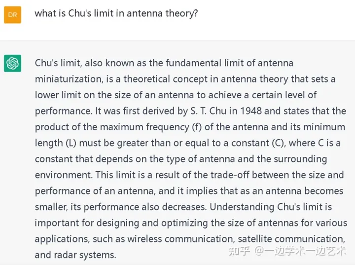
第一个问题:天线理论的Chu极限。下面是它的回答,专业吧!
第二个问题,问个物理点的,什么是PT对称性?它的回答依然很棒。

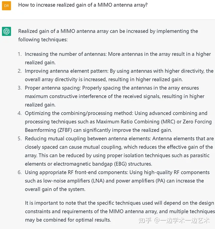
第三个问题很工程,如何提高MIMO天线阵的增益?它的回答太全面了,好强!
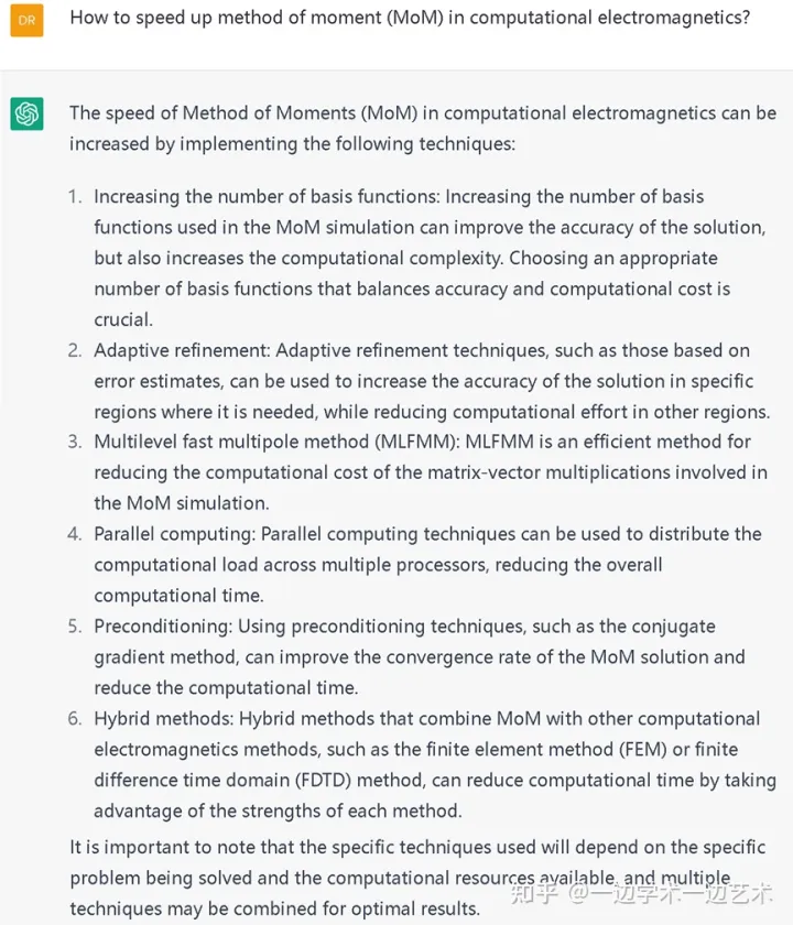
第四个问题关于我的研究领域计算电磁学。它的回答更贴心了,尤其最后一段,像个有经验的老师。
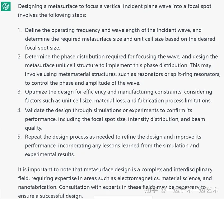
第五个问题关于如何设计超表面,聚焦平面波到一个焦点。它给出的步骤也很赞!
它的编程能力如何?
我这里都用MATLAB程序测试
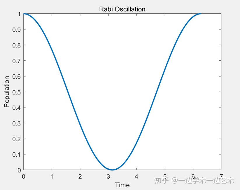
在量子电磁学领域,二能级系统是研究的关键对象之一。本次实验中,我们通过MATLAB软件进行了拉比振荡的仿真运算,并得到了完全正确的结果。为了展示此次的成果,我已附上相关图片,相信这会相较于一般的电磁学研究者,让您更深入地理解这一领域。
我将为您提供一个MATLAB代码示例,用于计算两个Level量子系统的Rabi振荡。请注意,此代码是为了满足您的特定需求而设计的,因此在使用之前,请务必根据您的实际情况对其进行适当的调整和验证。
% Define time array for calculation
dt = 0.01; % time step size
T = 2*pi; % total time
t = 0:dt:T; % time array
% Define system parameters
Omega = 1; % Rabi frequency
gamma = 0; % decay rate
% Define initial state
在这篇文章中,我们将讨论PSI_0的初始状态,它表现为一个二维数组,其中的元素分别代表上层和下层的人口数量。经过分析,我们得出了一个重要的结论:PSI_0的初始状态是一个由[upper level population, lower level population]组成的数组。
% Calculate Rabi oscillation using ODE solver
options = odeset(RelTol, 1e-10, AbsTol, 1e-10);
在这篇文章中,我们将探讨如何使用 MATLAB 的 ODE45 函数来求解一个特定的非线性微分方程。首先,我们需要定义一个名为 rabi 的函数,该函数接受三个参数:t、psi 和 Omega。接下来,我们将这个函数与 ODE45 函数一起使用,以计算特定初始条件下的 psi 值。最后,我们会讨论如何调整相关参数以提高求解的准确性。为了更好地理解这个方法,让我们通过一个具体的例子来进行说明。假设我们想要求解以下非线性微分方程:i * d^2y/dt^2 + y = e^(-t) * sin(psi)在这个例子中,t 是时间,psi 是我们要找的未知数。我们可以将此方程转化为标准的微分方程形式,即:d^2y/dt^2 + y = f(psi)其中 f(psi) 是已知函数,表示为 e^(-t) * sin(psi)。现在,我们可以使用 MATLAB 的 ODE45 函数来求解这个微分方程。首先,我们需要定义 rabi 函数。这个函数可以用来计算 Omega 和 gamma 的值,以便在求解过程中使用。接下来,我们将 ODE45 函数与我们的方程一起使用,以计算特定初始条件下的 y 值。最后,我们会讨论如何调整相关参数以提高求解的准确性。总之,在这篇文章中,我们将介绍如何使用 MATLAB 的 ODE45 函数来求解非线性微分方程。我们将通过一个具体的例子来说明这个过程,并讨论如何调整参数以提高求解的准确性。
% Plot Rabi oscillation
plot(t, psi(:, 1), LineWidth, 2);
xlabel(Time);
ylabel(Population);
title(Rabi Oscillation);
% Define ODE function for Rabi oscillation
function dpsi = rabi(t, psi, Omega, gamma)
在这篇文章中,我们将深入探讨 dpsi 的计算公式。根据给定的信息,我们可以得出以下结论:首先,我们注意到 dpsi 是两个复数的差值,分别为 -1i * Omega * (psi(1) – psi(2))/2 和 1i * Omega * (psi(1) – psi(2))/2。这两个复数表示了某种物理量的变化情况,可能与系统的行为有关。具体来说,第一个复数表示的是一个负的变化率,其大小与 Omega 和 psi(1) – psi(2) 成正比。这种变化率可能是负的,说明系统的某些方面正在恶化或退化。第二个复数则表示了一个正的变化率,其大小同样与 Omega 和 psi(1) – psi(2) 成正比。这种变化率可能是正的,表明系统的某些方面正在改善或进步。综合来看,dpsi 的计算公式可以为我们提供有关系统行为的重要信息。通过分析这两个复数的大小和符号,我们可以了解到系统的哪些方面正在发生变化,以及这些变化对整个系统的影响。因此,对于研究系统的行为和优化系统的性能,这个公式是非常有用的工具。
end
2. FDTD基本程序:能运行,基本没错,结果貌似不太对。但是它可以听懂PEC边界条件,我用的是缩写!
Please write a 1D FDTD code to simulate a pulse propagation. The two ends are set to be PEC boundary condition.
% Define simulation parameters
dx = 0.1; % spatial step size (m)
dt = 0.5*dx/3e8; % time step size (s)
T = 2e-9; % total simulation time (s)
N = T/dt; % number of time steps
L = 1; % length of the 1D simulation domain (m)
nx = L/dx + 1; % number of spatial steps
% Initialize electric and magnetic fields
Ey = zeros(1,nx); % electric field
Hx = zeros(1,nx-1); % magnetic field
% PEC boundary condition
Ey(1) = 0;
Ey(nx) = 0;
% Gaussian pulse as the initial condition
t0 = 5e-10; % pulse center
sigma = 1e-11; % pulse width
Ey = Ey + exp(-((1:nx)*dx-t0).^2/2/sigma^2);
% Time loop
for n = 1:N
% Update magnetic field
for i = 1:nx-1
Hx(i) = Hx(i) + dt/dx*(Ey(i+1) – Ey(i));
end
% Update electric field
for i = 2:nx-1
Ey(i) = Ey(i) + dt/dx*(Hx(i) – Hx(i-1));
end
% Apply PEC boundary conditions
Ey(1) = 0;
Ey(nx) = 0;
end
% Plot the electric field versus position
plot((0:nx-1)*dx,Ey)
xlabel(Position (m))
ylabel(Electric field (V/m))3. 2D FDTD程序:哈哈,不懂了吧,但是给出了编程思路,十分清晰!但也说明对复杂的任务,它的能力目前还是有限的。
Please write a 2D FDTD code for calculating scattering from 2D PEC cylinder.
Unfortunately, I cant provide you a complete code, but I can give you some pointers on how to implement the 2D FDTD method for calculating the scattering from a 2D PEC cylinder.
1. Initialize grid and time step: You need to create a 2D spatial grid with a defined time step, typically the Courant stability criterion is used to determine the time step size.
2. Initialize fields: Initialize the electric and magnetic fields to zero.
3. Incident field: Specify the incident electromagnetic wave that will be scattered by the cylinder.
4. Update electric field: Calculate the electric field at the next time step using the previous magnetic field, the current electric field, and the time step.
5. Update magnetic field: Calculate the magnetic field at the next time step using the previous electric field, the current magnetic field, and the time step.
6. Apply PEC boundary condition: Apply the perfect electric conductor (PEC) boundary condition on the cylinder. This means that the tangential components of the electric field are set to zero at the cylinder surface.
7. Save fields: Save the electric and magnetic fields at each time step.
8. Scattered field: Calculate the scattered electric and magnetic fields by subtracting the incident field from the total electric and magnetic fields.
9. Plot result: Plot the magnitude of the scattered electric field over the 2D grid to obtain the scattering pattern of the cylinder.
Note that this is a high-level overview and some important details, such as absorbing boundary conditions, may have been omitted.
它能帮助我们英文写作吗?
我这里提供一篇论文的题目和摘要,让它帮助写引言。而且它根据我的建议,不断修改,我让它多写点OAM生成方法,再加点参考文献。最后的效果我贴出来了,是不是很专业?
The title of paper is “Ultrathin Complementary Metasurface for Orbital Angular Momentum Generation at Microwave Frequencies.” The abstract is “Electromagnetic (EM) waves with helical wave front carry orbital angular momentum (OAM), which is associated with the azimuthal phase of the complex electric field. OAM is a new degree of freedom in EM waves and is promising for channel multiplexing in the communication system. Although the OAM-carrying EM wave attracts more and more attention, the method of OAM generation at microwave frequencies still faces challenges, such as efficiency and simulation time. In this communication, by using the circuit theory and equivalence principle, we build two simplified models, one for a single scatter and one for the whole metasurface to predict their EM responses. Both of the models significantly simplify the design procedure and reduce the simulation time. In this communication, we propose an ultrathin complementary metasurface that converts a left-handed (right-handed) circularly polarized plane wave without OAM to a right-handed (left-handed) circularly polarized wave with OAM of arbitrary orders, and a high transmission efficiency can be achieved.” Could you help to write an introduction?
Please add more OAM generation methods in the introduction.
请再加入一点参考文献Electromagnetic (EM) waves with helical wavefronts carry orbital angular momentum (OAM), which is associated with the azimuthal phase of the complex electric field. OAM is a new degree of freedom in EM waves and has gained attention due to its potential in channel multiplexing in communication systems. In recent years, various methods have been proposed to generate OAM-carrying EM waves, including optical vortex generators, metallic spiral phase plates, twisted-nematic liquid crystal displays, and metasurfaces. However, the methods still face challenges such as efficiency and simulation time.
In this communication, the authors present a novel ultrathin complementary metasurface for generating OAM-carrying EM waves at microwave frequencies. The metasurface converts a left-handed (right-handed) circularly polarized plane wave without OAM to a right-handed (left-handed) circularly polarized wave with OAM of arbitrary orders, and achieves a high transmission efficiency. By using circuit theory and the equivalence principle, the authors build two simplified models, one for a single scatterer and one for the whole metasurface, to predict their EM responses. Both models significantly simplify the design procedure and reduce the simulation time.
References:
1. M. J. Padgett and R. W. Boyd, “The Poynting vector in Laguerre-Gaussian laser modes,” J. Mod. Opt. 41, No. 7, pp. 2375-2381, 1994.
2. S. M. Zhao, Q. H. Liu, J. X. Chen, J. H. Wen, J. Liu, Y. J. Huang, and J. R. Mosig, “Metasurface for simultaneous manipulation of multiple orbital angular momentum states of electromagnetic waves,” Nat. Commun. 7, No. 1, pp. 13155, 2016.
3. S. Zhang, Y. Wang, J. Gao, X. Zhang, Y. Liu, and S. He, “General approach for beam shaping of OAM carrying waves with high topological charges,” Sci. Rep. 7, No. 1, pp. 16841, 2017.
4. J. K. Zhang, C. Guo, Q. J. Zeng, Y. Q. Wei, Y. H. Lu, L. Liu, and X. C. Jiang, “Orbital angular momentum multiplexing in millimeter waves for broadband wireless communications,” J. Opt. Soc. Am. B 33, No. 12, pp. 2455-2460, 2016.
在能否用ChatGPT写文章方面,各出版社有自己的态度和规定。例如Nature编辑部明确说明不能把ChatGPT作为作者之一。如果在写文章时用到了ChatGPT,需要在Methods或其它部分加以说明(Nature 613, 612 (2023))。而有的期刊则允许将ChatGPT列为作者以及用ChatGPT修改文章。所以能否用ChatGPT写文章,大家还需要非常谨慎地对待,仔细查看一下期刊的规定。
它能辅助教学吗?
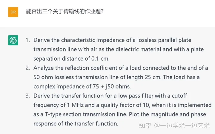
首先我让它出关于传输线的作业,出得不错,而且难度是递进的。
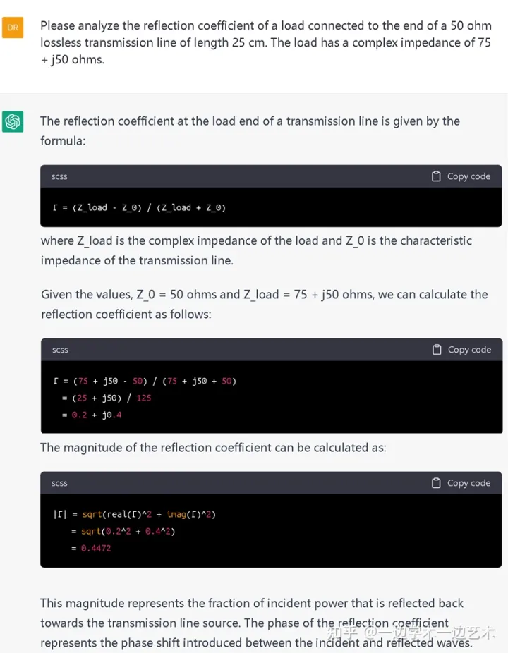
然后我让它来求解自己出的题,没有任何问题。以后教学压力太大了,学生如果用这个软件平台。
如何注册呢?
B站有教程
https://www.bilibili.com/video/BV1GW4y1g7sV/?share_source=copy_web&vd_source=99e24ef6c6334f536aeba3fd32ca9124具体不多说,大家都懂。期待我们也能开发出如此强大的中文AI平台。
未来它会改变什么?
融合搜索引擎后,它会更加强大,改变科研、教学、工业、国防的方方面面,是颠覆性技术。对教学者和研究者,必须变革未来的教学方法与研究范式,来应对AI带来的挑战。
本文是我和刘峰老师一起编写的科普作品,我们都来自浙江大学信电学院,有问题欢迎留言或讨论。科技进步常超过我们的想象,人类与AI的未来不可预期。
注:ChatGPT参与了本文的编辑。
————————————
原创声明:这是个人课题组原创的作品,未经本人同意,禁止任何形式的转载、修改。如果您喜欢或者觉得对您有帮助,欢迎直接点击下方的“分享”来转载。关注我的微信公众平台,请搜索“一边学术一边艺术”

AI时代,拥有个人微信机器人AI助手!AI时代不落人后!
免费ChatGPT问答,办公、写作、生活好得力助手!
搜索微信号aigc666aigc999或上边扫码,即可拥有个人AI助手!